Benchmark
File size, format read performance, and database comparisons — measured results and their limits.
The benchmark measures how much space a 3D city model takes in each format and what it costs to read it back with each format’s own reader. This page shows the results that exist today and names the parts that have not been measured yet.
What is measured
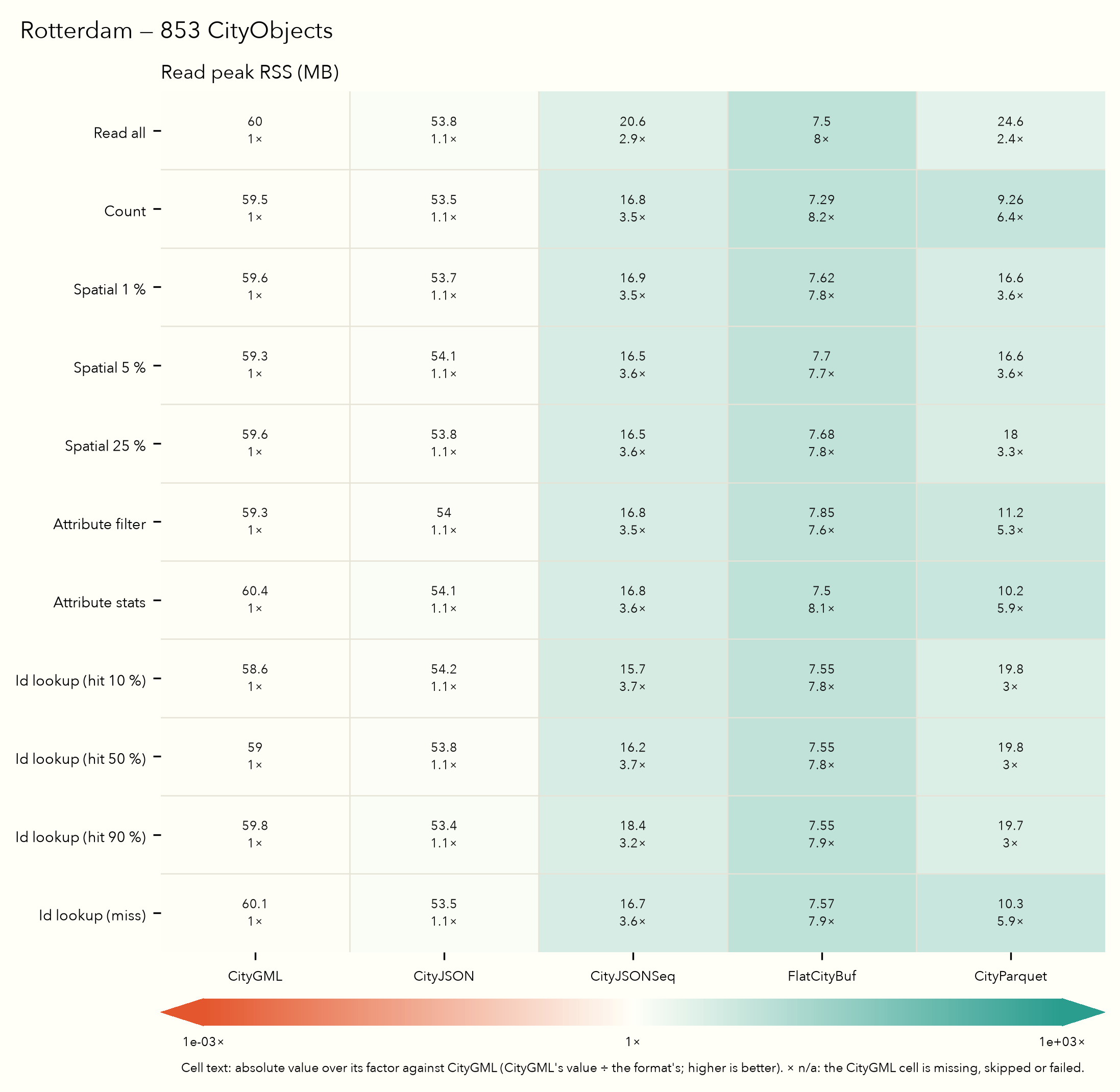
Five formats. CityGML 2.0, CityJSON, CityJSONSeq, FlatCityBuf and CityParquet (rows in Hilbert-curve order). CityGML is the baseline: every factor on this page is CityGML’s value divided by the format’s, so a larger factor is better (smaller, faster or leaner than CityGML).
Corpus. Six city datasets: Zurich (198,699 CityObjects), Tokyo (Chiyoda, 49,915), Montréal (31,415), New York (23,777), Vienna (1,322) and Rotterdam (853). Each dataset’s five artefacts derive from one normalised CityJSON source, which keeps one geometry per LoD and object and no semantic surfaces below LoD 2, so the corpus holds only content CityGML 2.0 can express. A 3DBAG slice of 1,000,001 CityObjects belongs to the corpus but has not been measured with the current harness.
Queries. Every format answers each query through its own mechanism and returns the same thing:
| Query | Returned by every format |
|---|---|
| Read all | Every record, all fields, in the format’s native form |
| Count | The number of objects |
| Spatial 1 %, 5 %, 25 % | Matching CityObjects, each with its highest-LoD geometry visited in place |
| Attribute filter | Count and identifiers of the CityObjects matching an attribute predicate |
| Attribute stats | Minimum, maximum, sum and count of a numeric attribute |
| ID lookup (×4) | One whole object, every field: hits at 10, 50 and 90 % of the file, a miss |
Appearance (textures and materials) is excluded for every format.
Protocol. Reads are warm-cache and single-threaded. Each cell runs one discarded warm-up and 25 timed samples, each in a fresh process; the figures report the median with the interquartile range, and peak resident memory. Sizes are on-disk bytes, in decimal units (1 MB = 10⁶ bytes).
File size
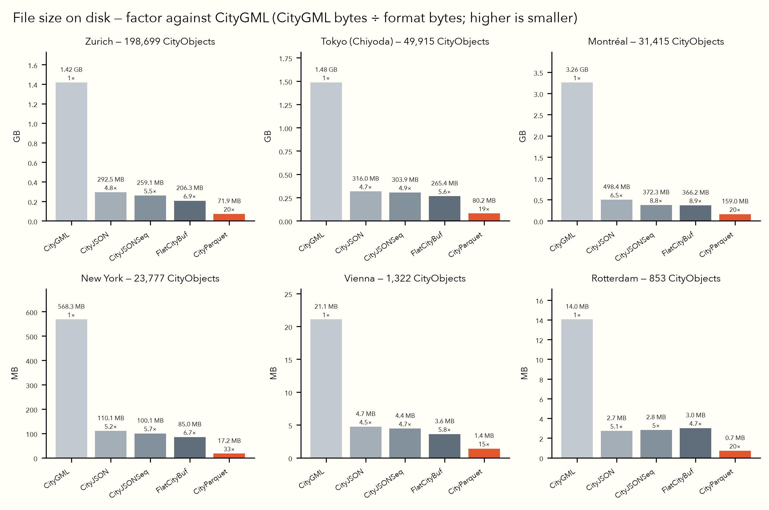
A file’s size is its length; a CityParquet package’s size is the sum of every file in its directory. The factor is CityGML bytes divided by CityParquet bytes.
| Dataset | CityObjects | CityGML | CityJSON | CityJSONSeq | FlatCityBuf | CityParquet | Factor |
|---|---|---|---|---|---|---|---|
| Zurich | 198,699 | 1.42 GB | 292.5 MB | 259.1 MB | 206.3 MB | 71.9 MB | 19.7× |
| Tokyo (Chiyoda) | 49,915 | 1.48 GB | 316.0 MB | 303.9 MB | 265.4 MB | 80.2 MB | 18.5× |
| Montréal | 31,415 | 3.26 GB | 498.4 MB | 372.3 MB | 366.2 MB | 159.0 MB | 20.5× |
| New York | 23,777 | 568.3 MB | 110.1 MB | 100.1 MB | 85.0 MB | 17.2 MB | 33.0× |
| Vienna | 1,322 | 21.1 MB | 4.7 MB | 4.4 MB | 3.6 MB | 1.4 MB | 15.1× |
| Rotterdam | 853 | 14.0 MB | 2.7 MB | 2.8 MB | 3.0 MB | 0.7 MB | 19.7× |
CityParquet is the smallest of the five formats on all six datasets, from 15.1× smaller than CityGML (Vienna) to 33.0× (New York). The ranking applies to these encodings and the writers’ default settings; it is not a claim about every format or compression configuration.
Format read timings
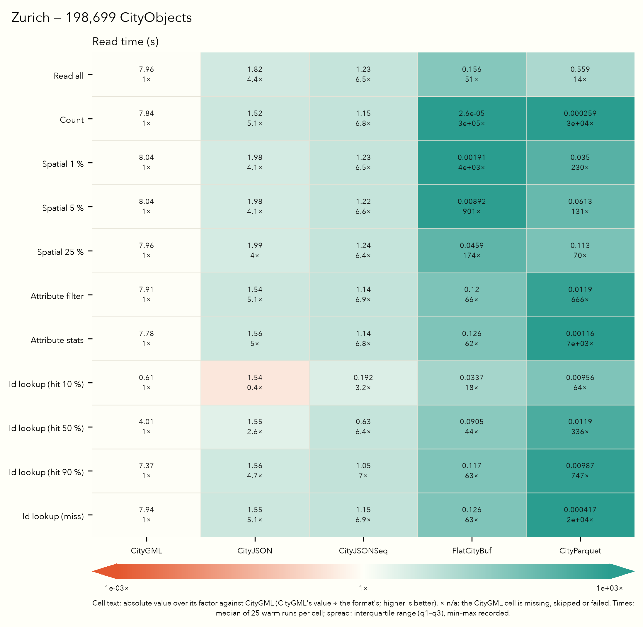
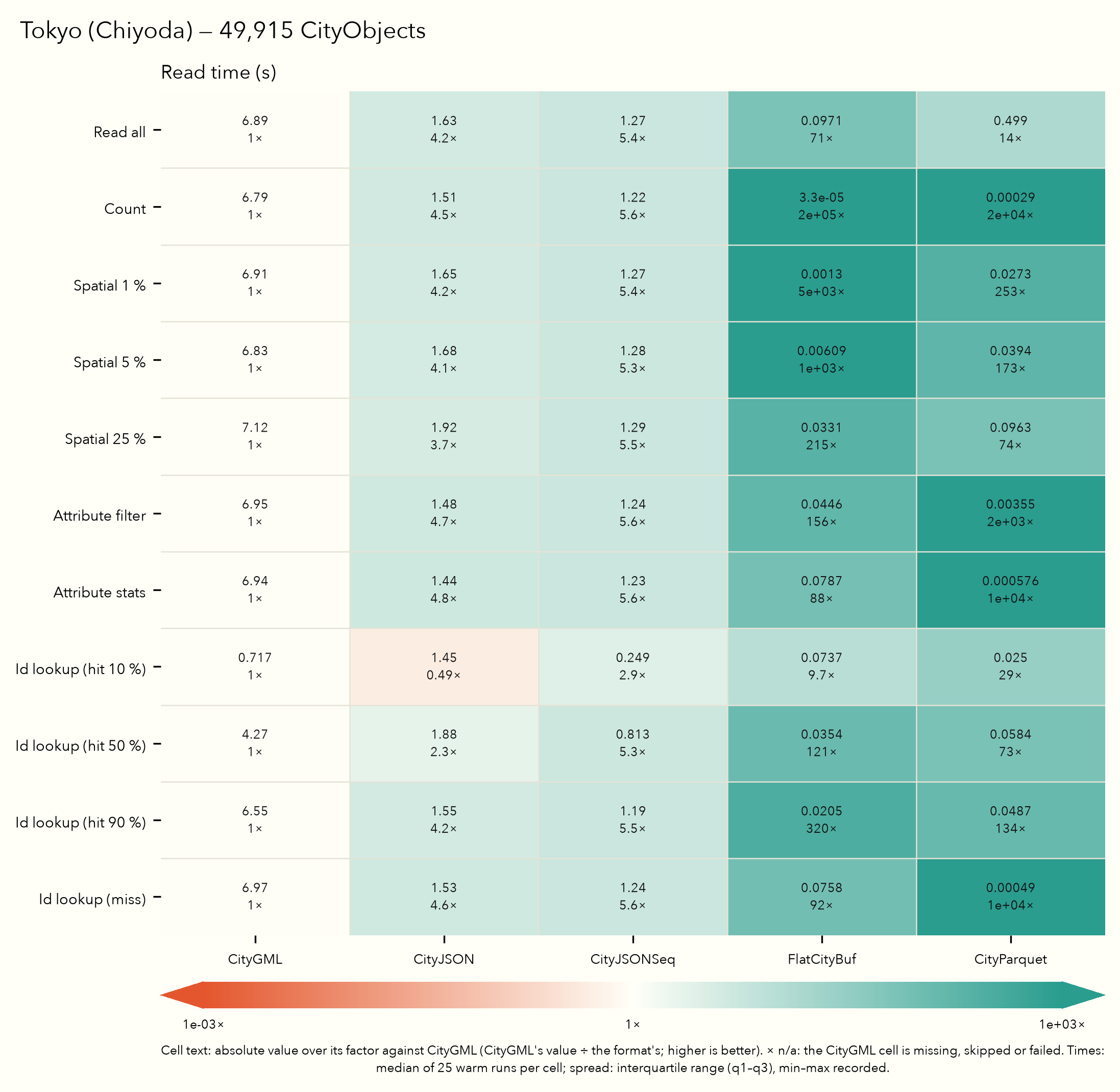
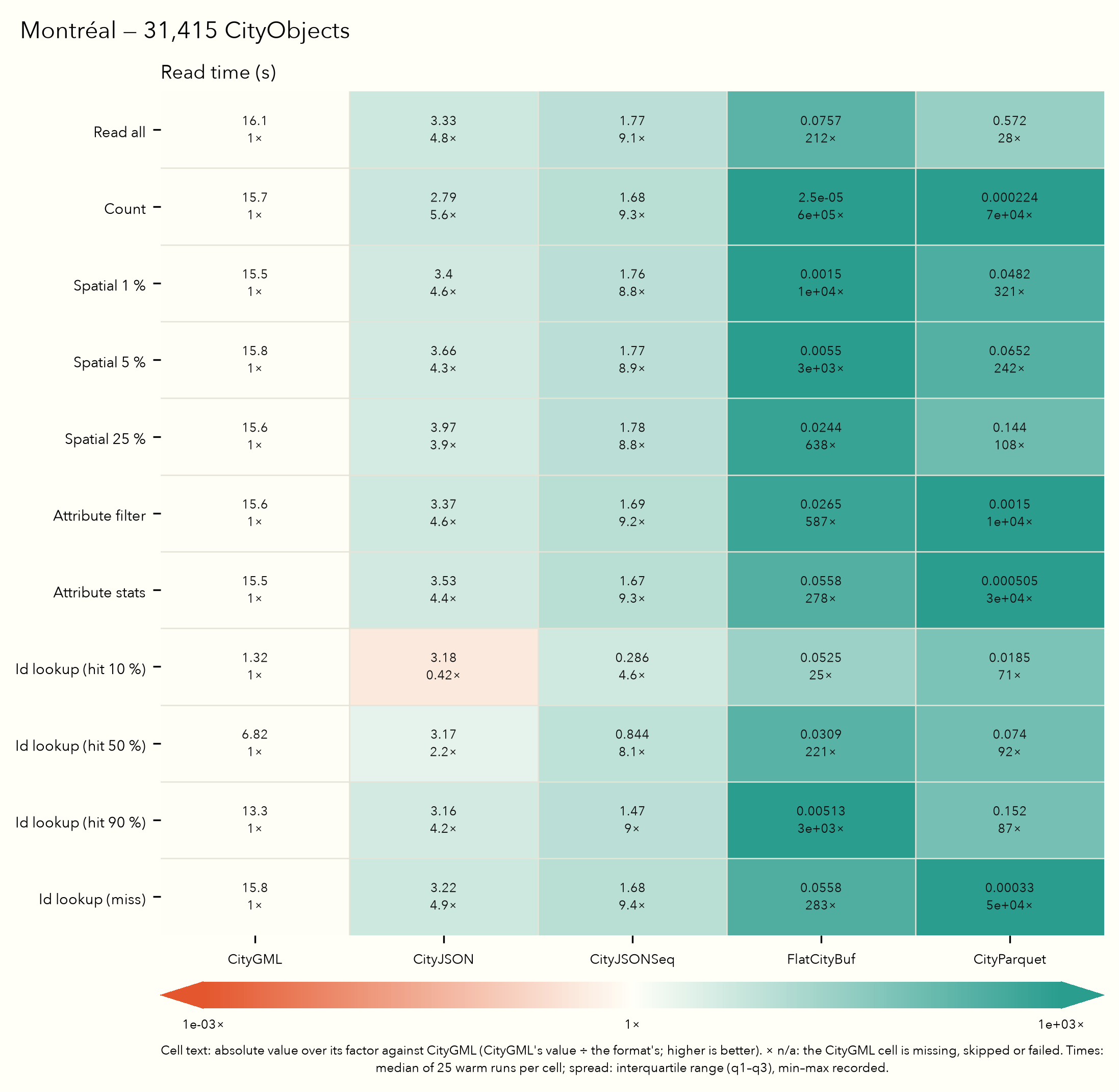
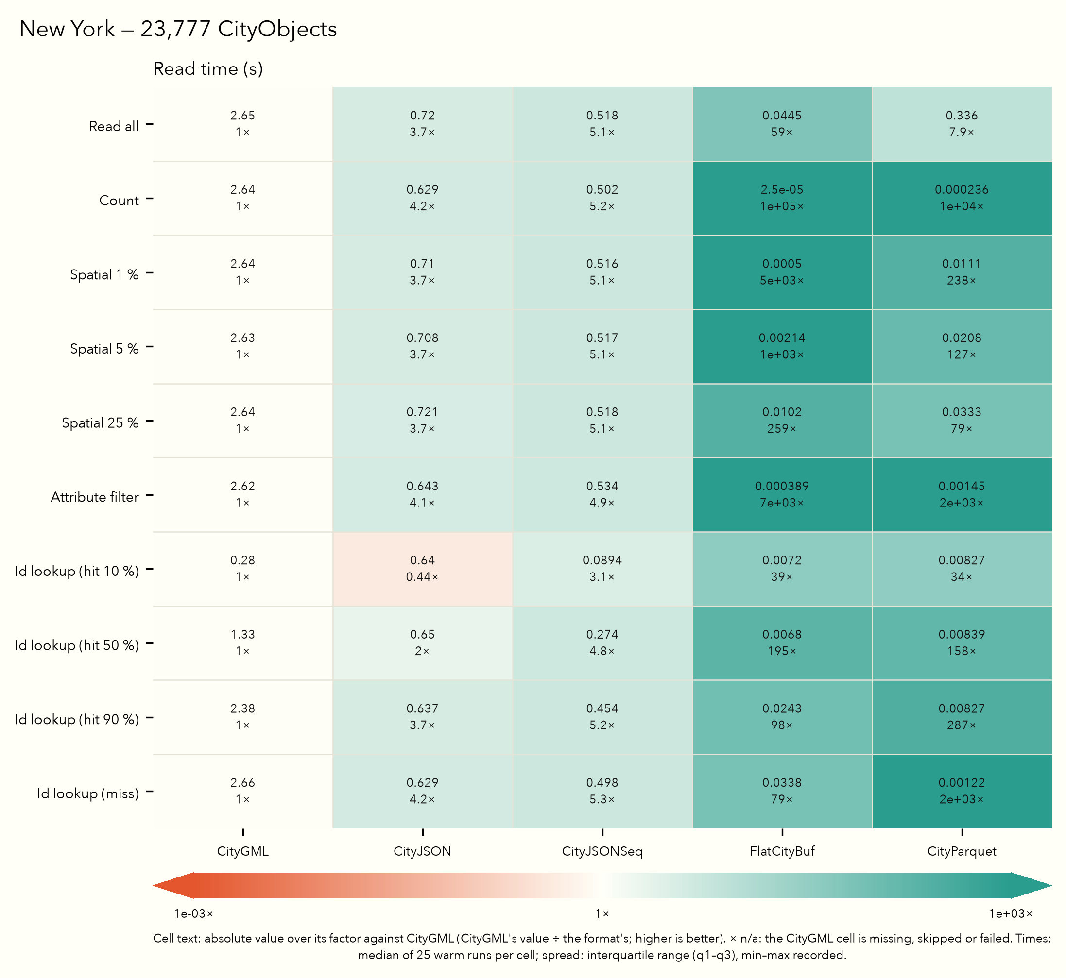
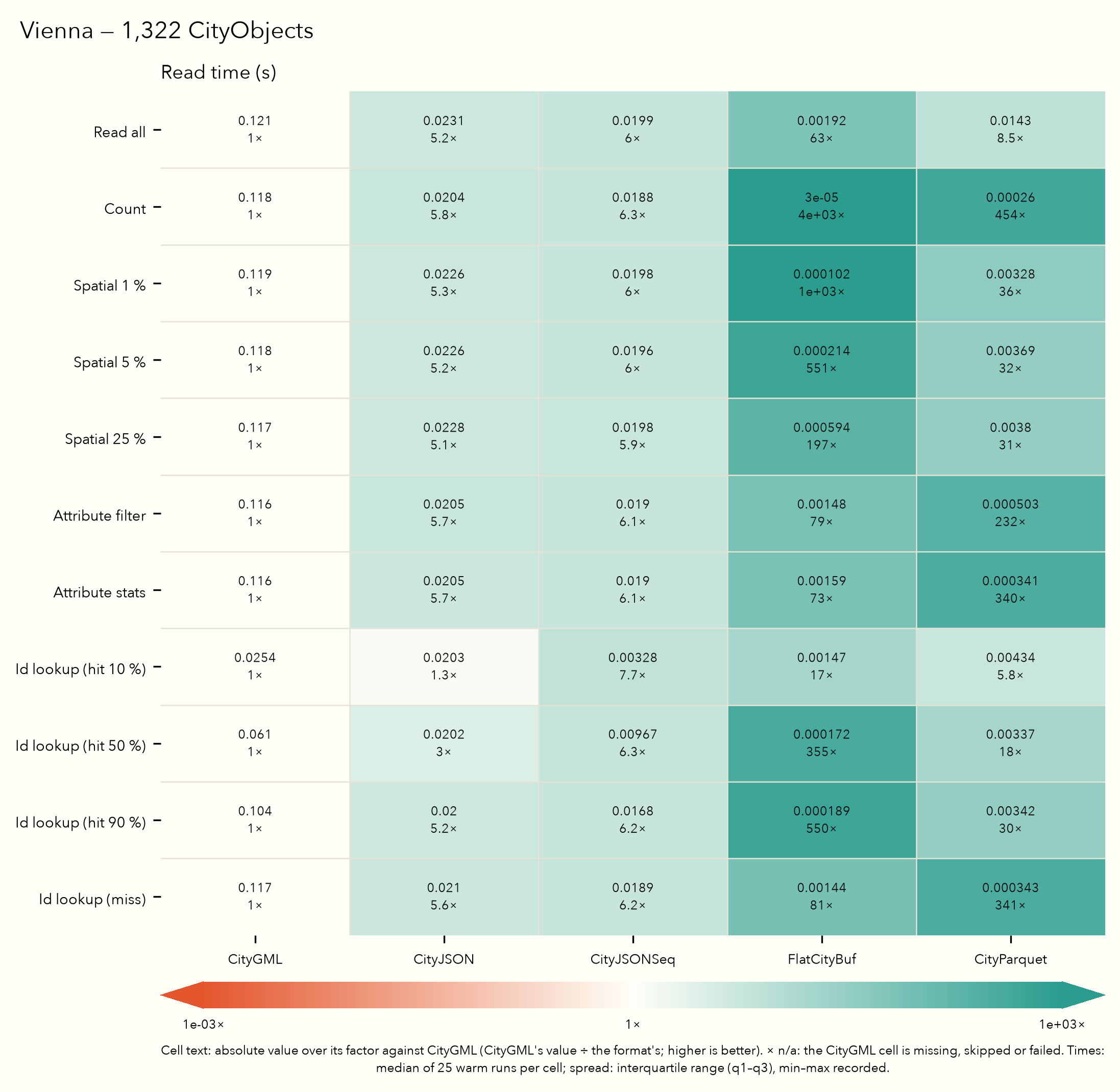
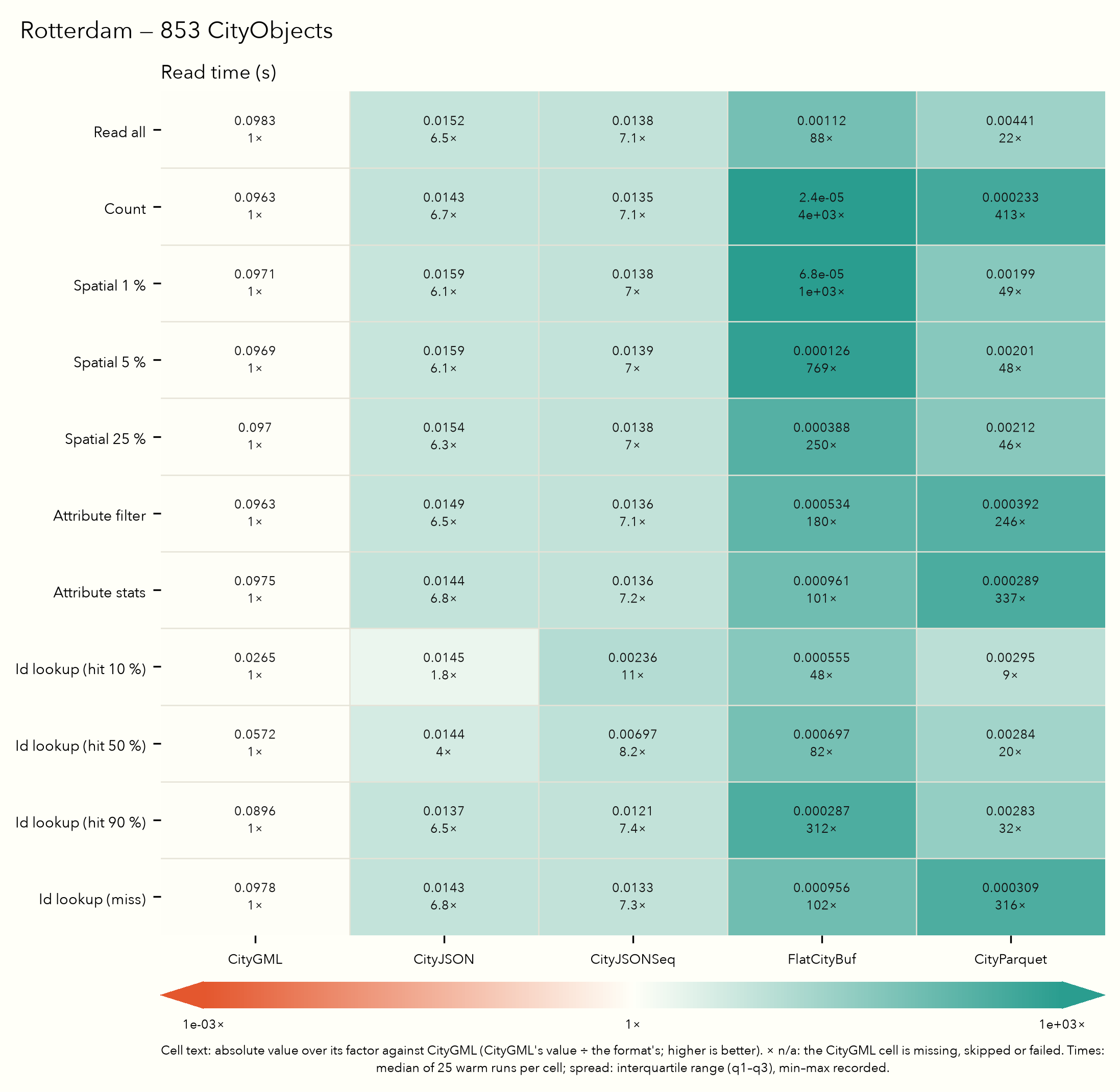
One figure per dataset: read time per query and format, each cell giving the median and its factor against CityGML.
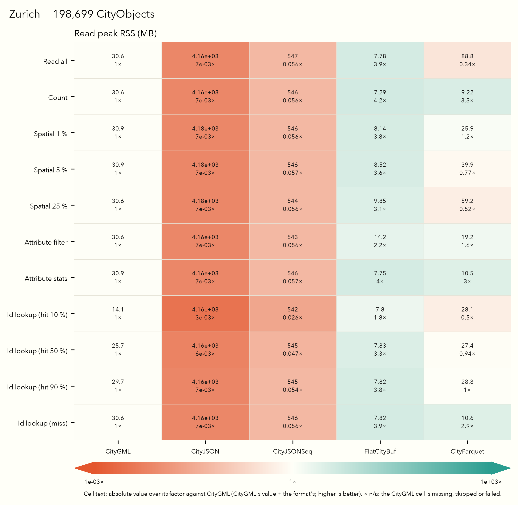
Peak memory, in the same layout: Zurich, Tokyo, Montréal, New York, Vienna, Rotterdam.
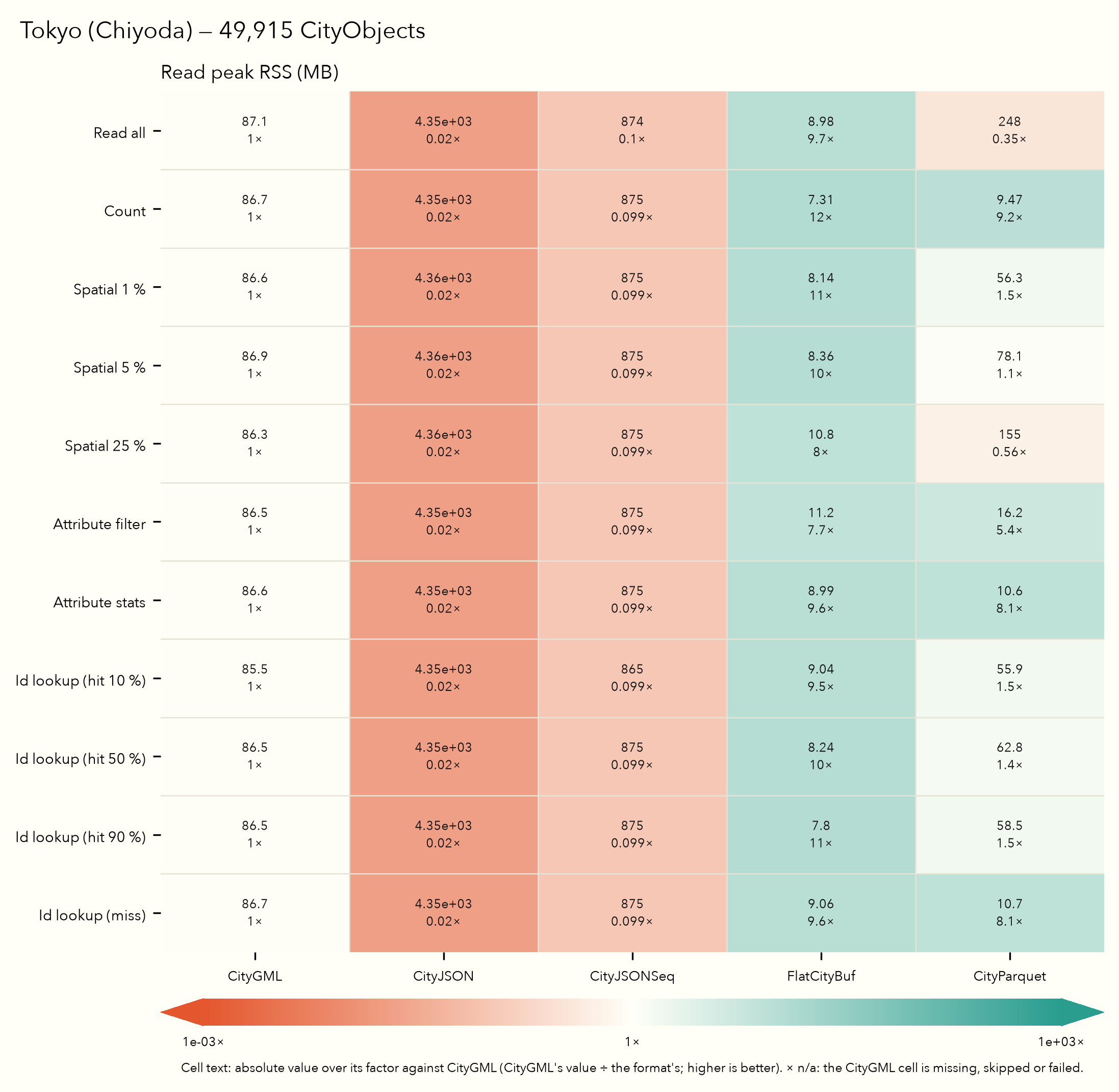
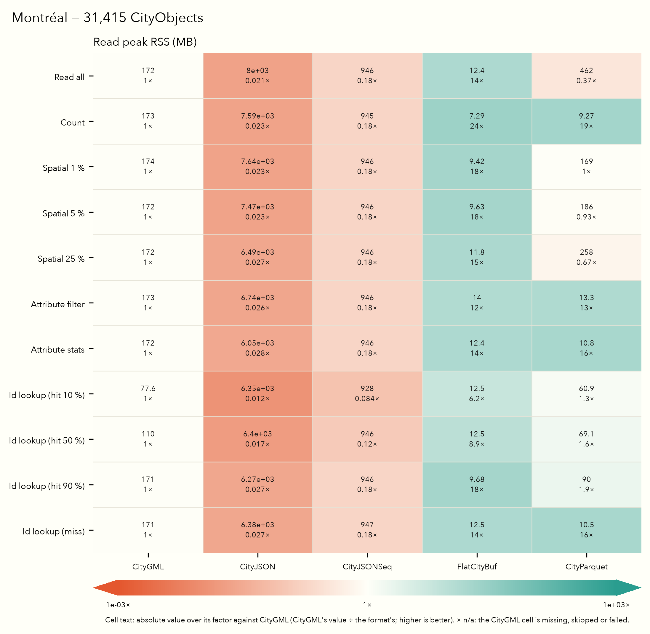
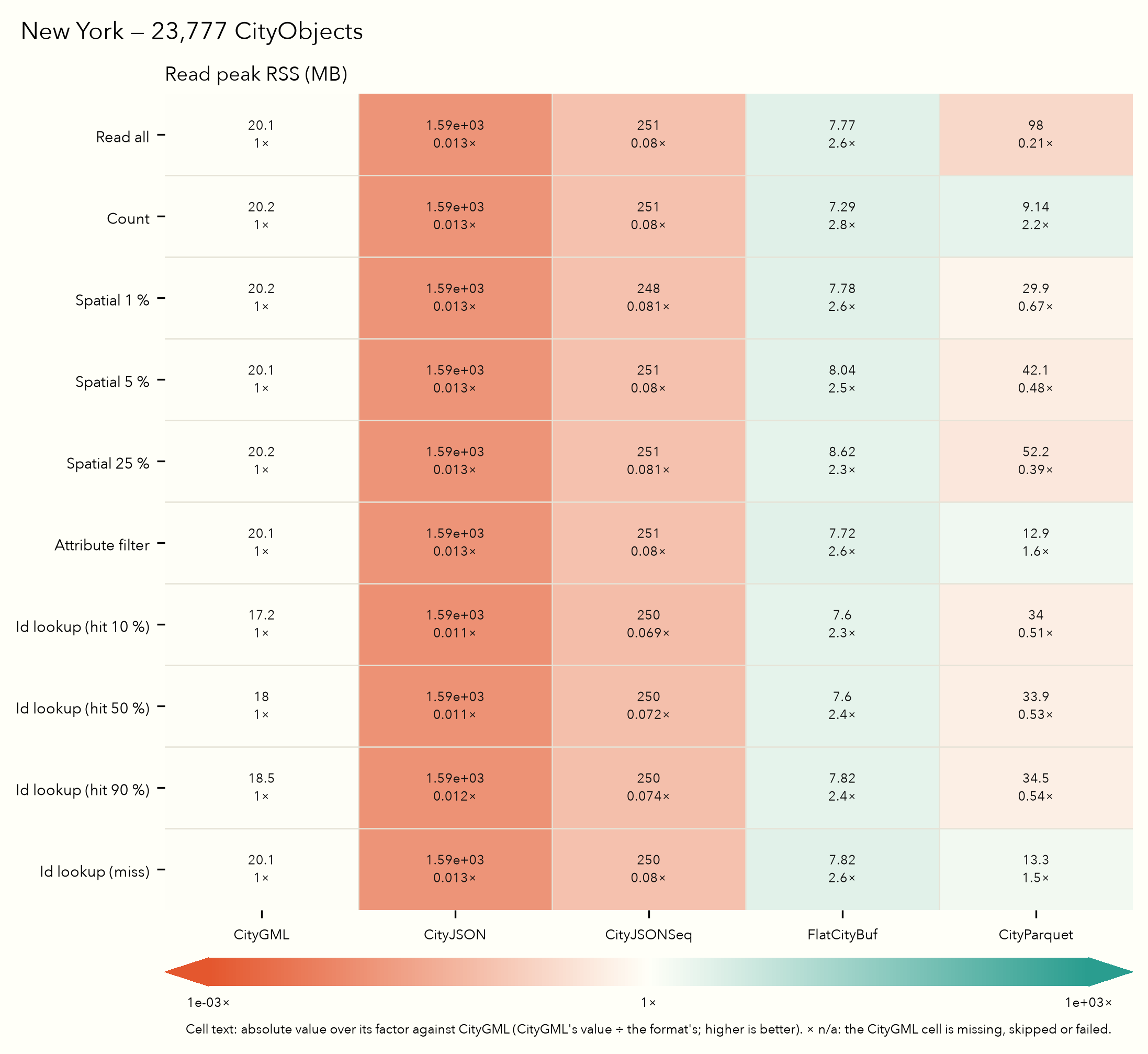
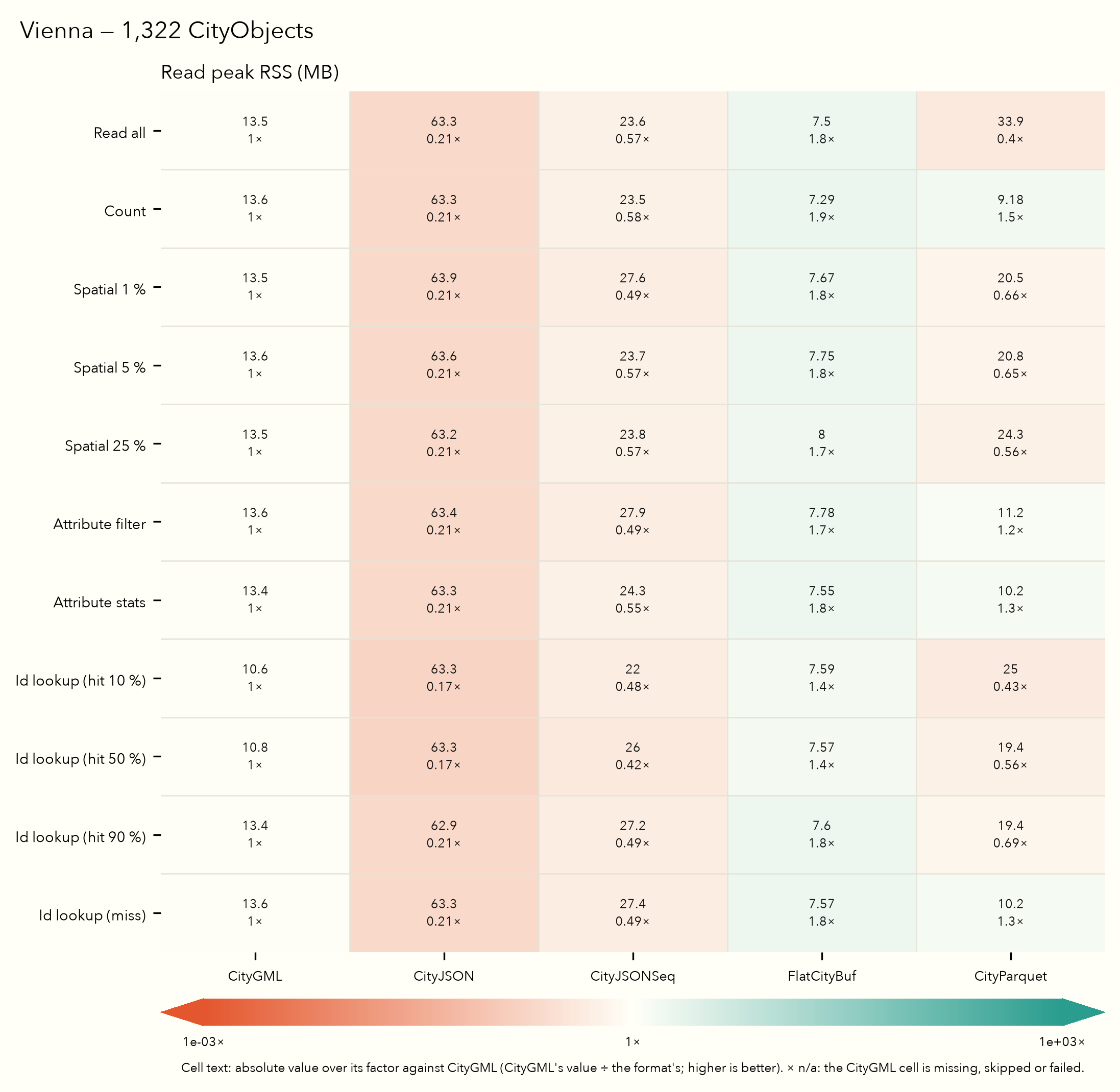
CityParquet is fastest where a query needs few columns. It answers the attribute statistics and the identifier miss fastest on every dataset measured, and the attribute filter on five of six. On Montréal in this run, the attribute filter took 1.5 ms with CityParquet, 26.5 ms with FlatCityBuf and 15.6 s with CityGML. On New York, FlatCityBuf’s attribute index answers the filter faster (0.39 ms against 1.45 ms); there the predicate is an identifier equality that matches 0.7 % of the objects. New York has no numeric attribute, so it has no attribute-statistics result.
FlatCityBuf is fastest on read all, count and every spatial window, on all six datasets. On Montréal in this run, read all took 0.076 s with FlatCityBuf and 0.57 s with CityParquet, and the 1 % window 1.5 ms and 48 ms. Both formats count in well under a millisecond, from a header or a footer. The identifier hits are mixed between the two and depend on where the object sits in the file.
CityParquet’s spatial window prunes nothing on five of the six datasets. At the writer’s default of 65,536 rows per row group, only Zurich spans more than one group, so the bounding-box statistics cannot skip any part of the other five packages. The window reads the identifier, bounding-box and geometry columns of every row in the groups it touches, so the whole geometry column is decompressed, and walks the WKB of the matches only. That is why the 1 % window costs CityParquet tens of milliseconds where FlatCityBuf’s R-tree answers in one or two.
The text formats scale with file size. CityGML, CityJSON and CityJSONSeq carry no index, so every query parses the whole file, except an identifier hit in CityGML and CityJSONSeq, which stops at the object. CityGML’s read all took 16.1 s on Montréal (3.26 GB) and 0.098 s on Rotterdam (14.0 MB) in this run.
Not yet measured
The following families exist in the harness. None has been measured with the current harness, so this page reports no numbers for them.
Bloom filters
A comparison of two CityParquet packages of the 3DBAG slice, one with Bloom filters and one without, on identifier, feature and attribute-equality lookups, each as a hit and a miss. It records size, lookup time, memory and how many row groups the filters and the min/max statistics rule out. Not yet measured with the current harness.
Database comparison
DuckDB reading CityParquet, compared with cjdb and 3DCityDB on the 3DBAG slice: stored size with and without indexes, query time and peak working memory, under a single-threaded and a parallel configuration. It compares whole systems, so its timings are not comparable with the format reads above. Not yet measured with the current harness.
Network
The format reads over HTTP: per query, the time, the bytes read and the number of HTTP requests, against a simulated network with fixed bandwidth and latency and against real object storage. Not yet measured with the current harness.
How to interpret the results
- Warm and single-threaded. Every sample is a fresh process reading from a warm page cache, on one thread; no format uses parallel decoding. These are local native reads, not HTTP or browser timings.
- Median of 25. Each cell reports the median of 25 timed samples after one discarded warm-up, with the interquartile range as its spread. Differences smaller than that spread are not findings.
- Memory is the reader’s peak RSS, not total system memory or the filesystem cache.
- Decimal units throughout: 1 MB = 10⁶ bytes, 1 GB = 10⁹ bytes.
- Isolation belongs to the host run. On the benchmark host the measured processes are pinned to one NUMA node, memory-capped and gated on host load, and each measure is recorded as applied or not. None was applied to the run on this page.
- Every format must return the same answer. After a run, the harness compares each query’s result count, the digest of the returned identifiers and the extent of the visited geometry across the five formats. A disagreement fails the run; no result on this page carries one.
- Counting grain. Read all and count report CityObjects in CityParquet and CityJSON but top-level features in CityGML, CityJSONSeq and FlatCityBuf. The spatial windows, the attribute queries and the identifier lookups count CityObjects in every format.
The implementation is experimental. See the format methodology and database methodology for reader behaviour, query definitions and the full list of caveats.
Reproduce
From the CityParquet repository:
just bench-prep
just bench-run
just bench-summary
bench-prep obtains the prepared inputs, bench-run measures them and
bench-summary renders existing results without measuring anything.
The figures on this page are copied unmodified from the rendered summary into
documents/public/benchmarks/, together with the
underlying data, the
completeness record, the three factor tables
(sizes,
size extremes,
queries) and a
provenance record naming the source run and every
file’s sha256. An update exports all of them together, keeps incomplete or
failed results visible, and rewrites the provenance record.
Open the complete benchmark summary for every figure
and the measurement caveats.